
The ISP Column
A monthly column on all things Internet
|
|
|
|
|
|
|
Other Formats:
|
|
|
|
June 2005
Geoff Huston
In looking back over some 30 years of experience with the Internet, the critical component of the internet protocol suite that has been the foundation of its success as the technology of choice for the global communications system is the Internet Protocol (IP) itself, working an overlay protocol that can span almost any form of communications media. But I would also like to nominate another contender for a critical role within IP, namely the reliable transport protocol that sits on top of IP, the Transmission Control Protocol (TCP), and its evolution over time. In supporting this nomination it is interesting to observe that the end-to-end rate-adaptive control algorithm that was adopted by TCP represented a truly radical shift from the reliable gateway-to-gateway virtual circuit flow control systems used by other protocols of similar vintage. Its also interesting to note that TCP is not designed to operate at any particular speed, but it attempts to operate at a speed that uses its fair share of all available network capacity along the network path. The fundamental property of the TCP flow control algorithm is that that it attempts to be maximally efficient while also attempting to be maximally fair.
In a world where network infrastructure capacity and complexity is related to network cost and delivered data is related to network revenue, TCP fits in well. TCP’s minimal assumptions about the capability of network components permit networks to be constructed using simple transmission capabilities and simple switching systems. 'Simple' often is synonymous with cheap and scalable, and there is no exception here. TCP also attempts to maximize data delivery through adaptive end-to-end flow rate control and careful management of retransmission events. In other words, TCP is an enabler for cheaper networking for both the provider and consumer. For the consumer the offer of fast cheap communications has been a big motivation in the uptake for demand for Internet-based services, and this, more than any other factor, has been the major enabling factor for the uptake of the Internet itself. 'Cheap' is often enough in this world, and TCP certainly helps to make data communications efficient and therefore cheap.
While TCP is highly effective in many networking environments, that does not mean that it is highly effective in all environments. For example:
In those wireless environments where there is significant wireless noise, TCP may confuse radio-based signal corruption and the corresponding packet drop with network congestion, and consequently the TCP session may back off its sending rate too early and back off for too long.
TCP will also back off too early when there is insufficient buffer space in the network's routers. This is a more subtle effect, but it is related to the coarseness of the TCP algorithm and the consequent burstiness of TCP packet sequences. These bursts, which will occur at up to twice the bottleneck capacity rate, are smoothed out by network buffers. Buffer exhaustion in the interior of the network will cause packet drop, which will cause the generation of a loss signal to the active TCP session, which will, in turn, either halve its sending rate or in the worst case reset the session state and restart with a single packet exchange. Particularly in wide area networks, where the end-to-end delay bandwidth product becomes a significant factor, TCP uses the network's buffers to sustain a steady state throughput which matches the available network capacity. Where the interior buffers are under-configured in memory it is not possible to even out the TCP bursts to continuously flow through the constrained point at the available data rate.
TCP also asks of its end hosts to have sufficient local capacity equal to the network capacity on the forward and reverse paths. The reason why is that TCP will not discard data until the remote end has reliably acknowledged it, so the sending host has to retain a copy of the data for the time it takes to send the data plus the time for the remote end to send the matching acknowledgement.
Even taking these limitations into account it’s true to say that TCP works amazingly well in most environments. Nevertheless, one area is proving to be a quite fundamental challenge to TCP as we know it, and that’s the domain of wide area, very high speed data transfer.
Very High Speed TCP
End host computers, even laptop computers these days, are typically equipped with gigabit Ethernet interfaces, have gigabytes of memory and internal data channels that can move gigabits of data per second between memory and the network interface. Current IP networks are constructed using multi-gigabit circuits and high capacity switches and routers (assuming that there is still a quantitative difference between these two forms of packet switching equipment these days!). If the end hosts and the network both can support gigabit transmissions then a TCP session should be able to operate end-to-end at gigabits per second, and achieve the same efficiency at gigabit speeds as it does at megabit speeds - right?
Well, no, not exactly!
This is not an obvious conclusion to reach, particularly when the TCP Land Speed Record is now at some 7Gbps across a distance that spans 30,000 km of network. What's going on?
Let head back to the basics of TCP to understand some of the issues with very high speed TCP. TCP operates in one of two states, that of slow start and congestion avoidance.
Slow start mode is TCP’s initial mode of operation in any session, as well as its ‘reset’ mode. In this mode, TCP sends two packets in response to each ack packet that advances the sender's window. In approximate terms (delayed acks notwithstanding) this allows TCP to double its sending rate in each successive lossless round trip time interval. The rate increase is exponential, effectively doubling each round trip time (RTT) interval, and the rate increase is bursty, effectively sending data into the network at twice the bottleneck capacity during this phase.
In the other operating mode, that of congestion avoidance, TCP sends an additional segment of data for each loss-free round trip time interval. This is an additive rate increase rather than exponential, increasing the sender's speed at the constant rate of one segment per round trip time interval.
TCP will undertake a state transition upon the detection of packet loss. Small scale packet loss (of the order of 1 or 2 packets per loss event) will cause TCP to halve its sending rate and enter congestion avoidance mode, irrespective of whether it was in this mode already. Repetition of this cycle gives the classic saw tooth pattern of TCP behaviour, and the related derivation of TCP performance as a function of packet loss rate. Longer sustained packet loss events will cause TCP to stop using the current session parameters and recommence the congestion control session using the restart window size and enter the slow start control mode once again.
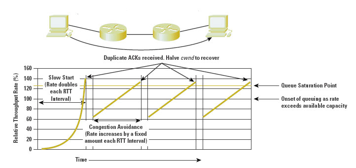
Figure 1 - TCP Behaviour
But what happens when two systems are at opposite sides of a continent with a high speed path between them? How long does it take for a single TCP session to get up to a data transfer rate of 10Gbps? Can a single session operate at a sustained rate of 10Gbps?
Lets look at a situation such as the network path from Brisbane, on the eastern side of the Australian continent to Perth on the western side. The cable path is essentially along the southern coast of the continent, so the round trip delay time (RTT) is 70ms. This implies that there are 14.3 round trip intervals per second. Lets also assume that the packet size being used is 1500 octets, or 12,000 bits, and the TCP initial window size is a single packet. Lets also assume that the bottleneck capacity of the host-to-host path between Brisbane and Perth is 10Gbps.
In a simple slow start model the sending speed doubles every 70ms, so after 17 RTT intervals where the sending rate has doubled for each interval, or after some 1.2 seconds have elapsed, the transfer speed has reached 11.2 Gbps (assuming a theoretical host with sufficiently fast hardware components, sufficiently fast internal data paths and adequate memory). At this stage lets assume that the sending rate will have exceeded the buffer capacity at the bottleneck point in the network path. Packet drop will occur as the critical point buffers in the network path have now saturated. At this point the TCP sender’s congestion window will halve, as will the TCP sending rate, and TCP will switch to congestion avoidance mode. In congestion avoidance mode the rate increase is 1 segment per RTT. This is equivalent to sending an additional 12Kbits per RTT, or, given the session parameters as specified above, this is equivalent to a rate increase of 171Kbps per second each RTT. So how long will it take TCP to recover and get back to a sending rate of 10Gbps?.
If this was a T-1 circuit where the available path bandwidth was 1.544Mbps, and congestion loss occurred at a sending rate of 2Mbps (higher than the bottleneck transmission capacity due to the effect of queuing buffers within the network), then TCP will rate halve to 1 Mbps and then use congestion avoidance to increase the sending rate back to 2Mbps. Within the selected parameters of a 70 ms RTT and 1500 byte segment size, this involves using congestion avoidance to inflate the congestion window from 6 segments to 12. This will take 0.42 seconds. So as long at the network can operate without packet loss for the session over an order of 1 second intervals, then TCP can comfortably operate at maximal speed in a megabit per second network.
What about our 10Gbps connection? The first estimate is the amount of useable buffer space in the switching elements. Assuming a total of some 256Mbytes of useable queue space on the network path prior to the onset of queue saturation, then the TCP session operating in congestion avoidance mode will experience packet loss some 590 RTT intervals after reaching the peak transmission speed of 10Gbps, or some further 41 seconds, at which point the TCP sending rate in congestion avoidance mode is 10.1Gbps. For all practical purposes the TCP congestion avoidance mode causes the sawtooth oscillation of this ideal TCP session between 5.0GBps and 10.1Gbps. A single iteration of this saw-tooth cycle will take 2,062 seconds, or 34 minutes and 22 seconds. The implication here is that the network has to be absolutely stable in terms of no packet loss along the path for time scales of the order of tens of minutes (or some billions of packets), and corresponding transmission bit error rates that are less than 10**-14. It also implies massive data sets to be transferred, as the amount of data passed in just one TCP congestion avoidance cycle is 1.95 terrabytes (1.95 x 10**12 bytes). Its also the case that the TCP session cannot make full use of the available network bandwidth, as the average data transfer rate is 7.55Gbps under these conditions, not 10Gbps.
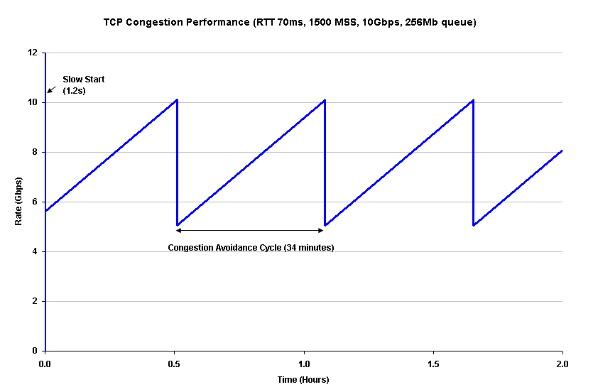
Figure 2 - TCP behaviour at High Speed
Clearly something is wrong with this picture, as it certainly looks like it's a hard and lengthy task to fill a long haul high capacity cable with data, and TCP is not behaving as we'd expect. While experimenting with the boundaries of TCP is in itself an interesting area of research, there are some practical problems here that could well benefit from this type of high speed transport.
TCP and the Land Speed Record
It is certainly possible to have TCP perform for sustained rates at very high speed, as the land speed records for TCP show, but something else is happening here, and there are a set of preconditions that need to be met before attempting to set a new record:
Firstly, its good, indeed essential, to have the network path all to yourself. Any form of packet drop is a major problem here, so the best way to ensure this is to keep the network path all to yourself!
Secondly its good, indeed essential to have a fixed latency. If the objective of the exercise is to reach a steady state data transmission then any change in latency, particularly because a reduction in latency has the risk of a period of over-sending, which in turn has a risk of packet loss. So keep the network as stable as possible.
Thirdly its essential to know in advance both the round trip latency and the available bandwidth.
You can then multiply these two numbers together (RTT and bandwidth), divide by the packet size, round down, and be sure to configure the sending TCP session to have precisely this buffer size, and the receiver to have a slightly larger size. And then start up the session.
The intention here is that TCP will use slow start to the point where the sender runs out of buffer space, and will continue to sit at this speed for as long as the sender, receiver and network path all remain in a very stable state. For the example configuration of a 10Gbps system with 70ms RTT, then setting a buffer limit of 116,000 packets will cause the TCP session to operate at 9.94Gbps. As long as the latency remains absolutely steady (no jitter), and as long as there is no other cross traffic, this sending rate can, in theory at any rate, be sustained indefinitely, with a steady stream of data packets being matched by a steady stream of ack packets.
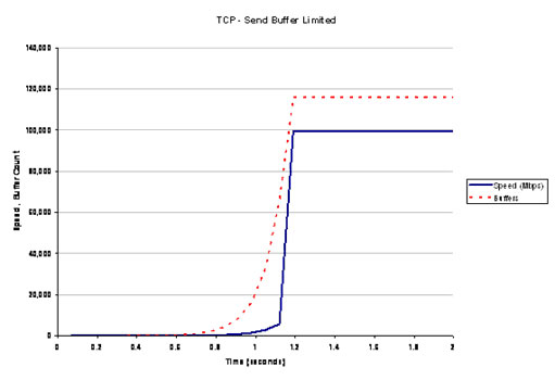
Figure 3 TCP operating with Buffer Saturation
Of course, this is an artificially constrained situation. The real issues here with the protocol are in the manner in which it shares a network path with other concurrent sessions as well as the protocol’s ability to fill the available network capacity. In other words, what would be good to see is a high speed high volume version of TCP that would be able to coexist on a network with all other forms of traffic, and, perhaps more ambitiously, that this high speed form of TCP can share the network fairly with other traffic sessions while at the same time making maximal use of the network. But TCP takes way too long in its additive increase mode (congestion avoidance) to recover one half of its original operating speed when operating at high speed across trans-continental sized network paths. If we want very high speed TCP to be effective and efficient then we need to look at changes to TCP for high speed operation.
High Speed TCP
There are two basic approaches to high speed TCP: parallelism of existing TCP, or changes to TCP to allow faster acceleration rates in a single TCP stream.
Using parallel TCP streams as a means of increasing TCP performance is an approach that has been around for some time. The original HTTP specification, for example, allowed the use of parallel TCP sessions to download each component of a web page (although HTTP 1.1 reverted to a a sequential download model because the overheads of session startup appeared to exceed the benefits of parallel TCP sessions in this case). Another approach to high speed file transfer through parallelism was that of GRID FTP. The basic approach is to split up the communications payload into a number of discrete components, and send each of these components simultaneously. Each component of the transfer may be between the same two endpoints (such as Grid FTP), or may be spread across multiple endpoints (as with BitTorrent).
But for parallel TCP to operate correctly you need to have already assembled all the data (or at a minimum know where all the data components are located). Where the data is being generated on the fly (such as observatories, or particle colliders) in massive quantities, there may be no choice but to treat the data set as a serial stream and use a high speed transport protocol to dispatch it. In this case the task is to adjust the basic control algorithms for TCP to allow it to operate at high speed, but also to operate ‘fairly’ on a mixed traffic high speed network.
Parallel TCP
Using parallelism as a key to higher speed is a common computing technique, and lies behind many supercomputer architectures. The same can apply to data transfer, where a data set is divided into a number of smaller chunks, and each component chunk is transmitted using its own TCP session. The underlying expectation here is that when using some number, N, of parallel TCP sessions, a single packet drop event will most probably cause the fastest of the N sessions to rate halve, as the fastest session will have more packets in flight in the network, and is therefore the most likely session to be impacted by a packet drop event. This session will then use congestion avoidance rate increase to recover. This implies that the response to a single packet drop is to reduce the sending rate by at most 1/(2N). For example, using 5 parallel TCP sessions, the response to a single packet drop event is to reduce the total sending rate by 1 / (2 x 5), or 1/10, as compared to the response from a single TCP session, where a single packet drop event would reduce the sending rate by 1/2.
An simulated version of 5 parallel sessions in a 10Gbps session is shown in Figure 4.
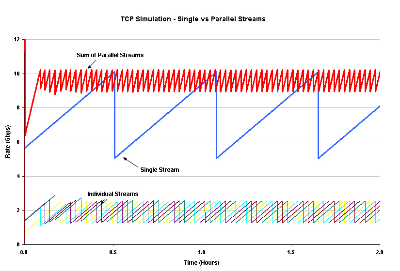
Figure 4 - Parallel TCP Simulation
The essential characteristics of the aggregate flow is that, under lossless conditions the data flow of N parallel sessions increases at a rate N times faster than a single session in congestion avoidance mode. Also the response to an isolated loss event is that of rate halving of a single flow, so that the total flow rate under ideal conditions is between R and R * (2N-1)/2N, or a long term average throughput of R * (4N-1)/4N. For N = 100 our theoretical 10Gbps connection could now operate at 9.9Gbps.
Of course the one major difference between theory and practice is that practice is different from theory, and there has been a considerable body of work looking at the performance of parallel TCP under various conditions, both in terms of maximizing throughput and the most efficient choice of the number of parallel active streams to use. Part of the problem is that while simple simulations, such as that used to generate Figure 4, tend to evenly distribute each of the parallel sessions to maximise the throughput, there is the more practical potential that the individual sessions self-synchronise. Because the parallel sessions have a similar range of window sizes, it is possible that at a given point in time there will be a similar number of packets in the network path from each stream. If the packet drop event is a multiple packet drop event, such as a tail-drop queue, then it is entirely feasible that a number of parallel streams will experience packet loss simultaneously, and there is the consequent potential for the streams to fall into synchronization.
The two extremes, evenly distributed and tightly synchronized multiple streams are indicated in Figure 5. The average throughput of parallel synchronized streams is the same as a single stream over extended periods in this simulation, and both are certainly far worse than an evenly distributed set of parallel streams.
One way to address this problem is to reunite these parallel streams into a single controlled stream that exhibits the same characteristics as evenly spread parallel streams. This approach, MulTCP, is considered in the next section.
And it all this analysis of parallel TCP streams sounds a little academic and unrelated to networking today, its useful to note that many ISPs these days see BitTorrent traffic as their highest volume application these days. Bit Torrent is a peer-to-peer protocol that undertakes transfer of datasets using a highly parallel transfer technique. Under BitTorrent the original data set is split into blocks, each of which may be downloaded in parallel. The subtle twist here is that the individual sessions do not have the same source points, and the host may take feeds from many different sources simultaneously, as well as offering itself as a feed point for the already downloaded blocks. This behaviour exploits the peer-to-peer nature of these networks to a very high extent, potentially not only exploiting parallel TCP sessions for speed gains, but also exploiting diverse network paths and diverse data sources to avoid single path congestion. Considering its effectiveness in terms of maximizing transfer speeds for high volume data sets and its relative success in truly exploiting the potential of peer-to-peer networks, and of course the dramatic uptake of BitTorrent and its extensive use, BitTorrent probably merits closer examination, but perhaps that’s for another time and an article all on its own.
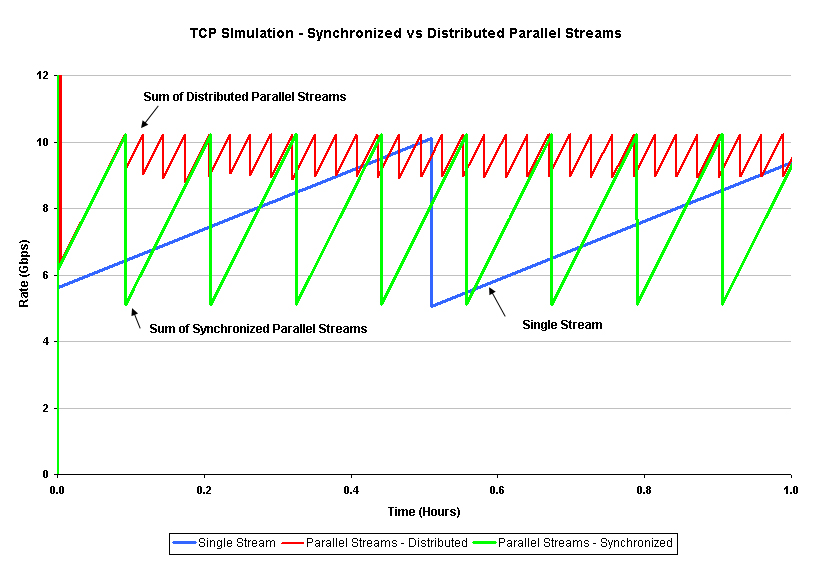
Figure 5 - Comparison of Parallet TCP - Synchronized and
Distributed Streams
Very High Speed Serial TCP
The other general form of approach is to re-examine the current TCP control algorithm to see if there are parameter or algorithm changes that could allow TCP to undertake a better form of rate adaptation to these high capacity long delay network paths. The aim here is to achieve a good congestion response algorithm that does not amplify transient congestion conditions into sustained disaster areas, while at the same time being able to support high speed data transfers making effective use of all available network capacity. Also on this wish list is a desire to behave sensibly in the face of other TCP sessions, so that it can share the network with other TCP sessions in a fair manner.
MulTCP
The first of these approaches is MulTCP. This is a single TCP stream that behaves in a manner equivalent to N parallel TCP sessions, where the virtual sessions are evenly distributed in order to achieve the optimal outcome in terms of throughput. The essential changes to TCP are in congestion avoidance mode and the reaction of packet loss. In congestion avoidance mode MulTCP increases its congestion window by N segments per RTT, rather than the default of a single segment. Upon packet loss MulTCP reduces its window by W/(2N), rather than the default of W/2. MulTCP uses a slightly different version of slow start, increasing its window by 3 segments per received ACK, rather than the default value of 2.
MulTCP represents a simple change to TCP that does not depart radically from TCP’s congestion control algorithm. Of course choosing an optimal value for N is one where some understanding of the network characteristics would help. Too high a value for N and the MulTCP session has a tendency to claim an unfair amount of network capacity, while too small a value for N does not necessarily take full advantage of available network capacity. Figure 6 shows MulTCP compared to a simulation of an equivalent number of parallel TCP streams and a single TCP stream (N = 5 in this particular simulation).
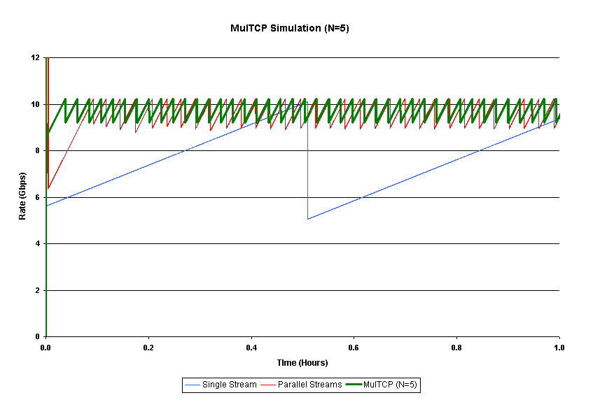
Figure 6 - MulTCP
Good as this is, there is the lingering impression that we can do better here. It would be better not to have to configure the number of virtual parallel sessions. It would be better to support fair outcomes when competing with other concurrent TCP sessions over a range of bandwidths, and it would be better to have a wide range of scaling properties. There is no shortage of options here for tweaking various aspects of TCP to meet some of these preferences, ranging from adaptations applied to the TCP rate control equation to approaches that view the loading onto the network as a power spectrum problem.
HighSpeed TCP
Another approach, described in RFC 3649, "HighSpeed TCP for Large Congestion Windows" looks at this from the perspective of the TCP rate equations, developed by Sally Floyd at ICIR.
When TCP operates in congestion avoidance mode at an average speed of W packets per RTT, then the number of packets per RTT varies between (2/3)W and (4/3)W. Each cycle takes (2/3)W RTT intervals, and the number of packets per cycle is therefore (2/3)W2 packets. This implies that the rate can be sustained at W packets per RTT as long as the packet loss rate is 1 packet loss per cycle, or a loss rate, p, where p = 1/((2/3)W**2). Solving this equation for W gives the average packet rate per RTT of W = sqrt(1.5) / sqrt(p). The general rate function for TCP, R, is therefore R = (MSS/RTT) * (sqrt(1.5) / sqrt(p)), where MSS is the TCP packet size.
Taking this same rate equation approach, what happens for N multiple streams? The ideal answer is that the parallel streams operate N times faster at the same loss rate, or, as a rate equation the number of packets per RTT, Wn, can be expressed as Wn = N((sqrt(1.5) / sqrt(p)), and each TCP cycle is compressed to an interval of (2/3) (Wn**2/N**2).
But perhaps the desired response is not to shift the TCP rate response by a fixed factor of N, as is the intent with MulTCP, but to adaptively increase the sending rate through increasing values of N as the loss rate falls. The proposition made by HighSpeed TCP is to propose a TCP response function that preserves the fixed relationship between the logarithm of the sending rate and the logarithm of the packet loss rate, but alters the slope of the function, such that TCP increases its congestion avoidance increment as the packet loss rate falls. This relationship is shown in Figure 7, where the log of the sending rate is compared to the log of the packet loss rate. MulTCP preserves the same relationship between the log of the sending rate and the log of the packet loss rate, but alters the offset, while changing the value of the exponent of the packet loss rate causes a different slope to the rate equation.
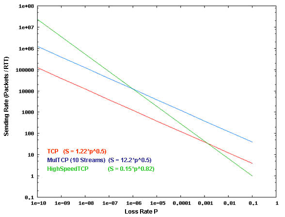
Figure 7 - TCP Response Functions
One way to look at the HighSpeed TCP proposal is that it operates in the same fashion as a turbo-charger on an engine; the faster the engine is running, the higher the turbo-charged boost to the engine’s normal performance. Below a certain threshold value the TCP congestion avoidance function is unaltered, but once the packet loss rate falls below a certain threshold value then the higher speed congestion avoidance algorithm is invoked. The higher speed rate equation proposed by HighSpeed TCP is based on achieving a transfer rate of 10Gbps over a 100ms latency path with a packet loss rate of 1 in 10 million packets . Working backward from these parameters gives us a rate equation for W, the number of packets per RTT interval of W = 0.12 / p0.835. This is approximately equivalent to a MulTCP session where the number of parallel sessions, N, is raised as the TCP rate increases.
This can be translated into two critical parameters for a modified TCP: the number of segments to be added to the current window size for each lossless RTT time interval, and the number of segments to reduce the window size in response to a packet loss event. Conventional TCP uses values of 1 and (˝)W respectively. The HighSpeed TCP approach increases the congestion window by 1 segment for TCP transfer rates up to 10Mbps, but then uses an increase of some 6 segments per RTT for 100Mbps, 26 segments at 1Gbps and 70 segments at 10Gbps. In other words the faster the TCP rate that has already been achieved achieved, then the greater the rate acceleration. Highspeed TCP also advocates a smaller multiplicative decrease in response to a single packet drop, so that at 10Mbps the multiplier would be 1/2, at 100Mbps the multiplier is 1/3, 1Gbps it is 1/5 and at 10Gbps it is set to 1/10.
What does this look like? Figure 8 shows a HighSpeed TCP simulation. What is not easy to discern is during congestion avoidance HighSpeed TCP opens its sending window in increments of 61 through 64 each RTT interval, making the rate curve slightly upward during this window expansion phase. HighSpeed TCP manages to recover from the initial rate halving from slow start in around 30 seconds, and operates at a 8 second cycle, as compared to a single TCP stream’s 38 minute cycle, or a N stream MulTCP session that operates at a 20 second cycle.
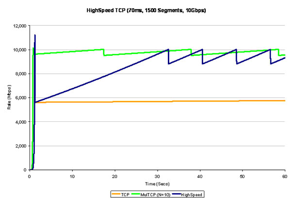
Figure 8 = HighSpeed TCP Simulation
One other aspect of this work concerns the so-called slow start algorithm, which at these speeds is not really slow at all. The final round trip time interval in our scenario has TCP attempting to send an additional 50Mbytes of data in just 70 ms. That’s an additional 33,333 packets that are pushed into the network’s queues. Unless the network path was completely idle at this point its likely that hundreds, if not thousands of these packets will be dropped in this step, pushing TCP back into a restart cycle. HighSpeed TCP has proposed a limited slow start to accompany HighSpeed TCP that limits the inflation of the sending window to a fixed upper rate per RTT to avoid this problem of slow start overwhelming the network and causing the TCP session to continually restart. Other changes for HighSpeed TCP are to extend the limit of three duplicate ACKs before retransmitting to a higher value, and a smoother recovery when a retransmitted packet is itself dropped.
Scaleable TCP
Of course HighSpeed TCP is not the only offering in the high performance TCP stakes.
Scalable TCP, developed by Tom Kelly at Cambridge University, attempts to break the relationship between TCP window management and the RTT time interval. It does this by noting that in ‘conventional’ TCP, the response to each ack in congestion avoidance mode is to inflate the sender’s congestion window size (cwnd) by (1/cwnd), thereby ensuring that the window in inflated by 1 segment each RTT interval. Similarly the window halving on packet loss can be expressed as a reduction in size by (cwnd/2). Scalable TCP replaces the additive function of the window size by the constant value a. The multiplicative decrease is expressed as a fraction b, which is applied to the current congestion window size.
In Scalable TCP, for each ack the congestion window is inflated by the constant value a, and upon packet loss the window is reduced by the fraction b. The relative performance of Scalable TCP as compared to conventional TCP and MulTCP is shown in Figure 9.
The essential characteristic of Scalable TCP is the use of a multiplicative increase in the congestion window, rather than a linear increase. This effectively creates a higher frequency of oscillation of the TCP session, probing upward at a higher rate and more frequently than HighSpeed TCP or MulTCP. The frequency of oscillation of Scalable TCP is independent of the RTT interval, and the frequency can be expressed as f = log(1 - b) / log(1 + a). In this respect longer networks paths exhibit similar behaviour to shorter paths at the bottleneck point. Scalable TCP also has a linear relationship between the log of the packet loss rate and the log of the sending rate, with a greater slope of HighSpeed TCP.
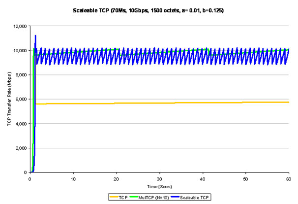
Figure 9 - Scaleable TCP
BIC and CUBIC
The common issue here is that TCP under-performs in those areas of application where there is a high bandwidth-delay product. The common problem observed here is that the additive window inflation algorithm used by TCP can be very inefficient in long delay high speed environments. As can be seen in Figure 10, the ACK response for TCP is a congestion window inflation operation where the amount of inflation of the window is a function of the current window size and some additional scaling factor.
BIC (Binary Increase Congestion Control) takes a different view, by assuming that TCP is actively searching for a packet sending rate which is on the threshold of triggering packet loss, and uses a binary chop search algorithm to achieve this efficiently. When BIC performs a window reduction in response to packet drop, it remembers the previous maximum window size, as well as the current window setting. With each lossless RTT interval BIC attempts to inflate the congestion window by one half of the difference between the current window size and the previous maximum window size. In this way BIC quickly attempts to recover from the previous window reduction, and, as BIC approaches the old maximum value, it slows down its window inflation rate, halving its rate of window inflation each RTT. This is not quite so drastic as it may sound, as BIC also uses a maximum inflation constant to limit the amount of rate change in any single RTT interval. The resultant behaviour is a hybrid of a linear and a non-linear response, where the initial window inflation after a window reduction is a linear increase, but as the window approaches the previous point where packet loss occurred the rate of window increase slows down. BIC uses the complementary approach to window inflation once the current window size passes the previous loss point. Initially further window inflation is small, and the window inflation value doubles in size for each RTT, up to a limit value, beyond which the window inflation is once more linear.
BIC can be too aggressive in low RTT networks and in slower speed situations, leading to a refinement of BIC, namely CUBIC. CUBIC uses a 3rd order polynomial function to govern the window inflation algorithm, rather than the exponential function used by BIC. The cubic function is a function of the elapsed time since the previous window reduction, rather than BIC’s implicit use of an RTT counter, so that CUBIC can produce fairer outcomes in a situation of multiple flows with different RTTs. CUBIC also limits the window adjustment in any single RTT interval to a maximum value, so the initial window adjustments after a reduction is linear. Here the new window size, W, is calculated as W = C(t – K)3 + Wmax, where C is a constant scaling factor, t is the elapsed time since the last window reduction event, Wmax is the size of the window prior to the most recent reduction and K is a calculated value: K = (Wmax ß / C)1/3. This function is more stable when the window size approaches the previous window size Wmax. The use of a time interval rather than an RTT counter in the window size adjustment is intended to make CUBIC more sensitive to concurrent TCP sessions, particularly in short RTT environments.
Figure 10 shows the relative adjustments for BIC and CUBIC, using a single time base. The essential difference between the two algorithms is evident in that the CUBIC algorithm attempts to reduce the amount of change in the window size when near the value where packet drop was previously encountered.
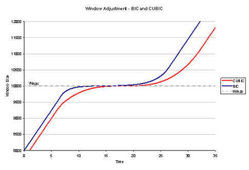
Figure 10 - Windows adjustment for BIC and CUBIC
Westwood
The ‘steady state’ mode of TCP operation is one that is characterized by the ‘sawtooth’ pattern of rate oscillation. The additive increase is the means of exploring for viable sending rates while not causing transient congestion events by accelerating the sending rate too quickly. The multiplicative decrease is the means by which TCP reacts to a packet loss event which is interpreted as being symptomatic of network congestion along the sending path.
BIC and CUBIC concentrate on the rate increase function, attempting to provide for greater stability for TCP sessions as they converge to a long term available sending rate. The other perspective is to examine the multiplicative decrease function, and see if there is further information that a TCP session can use to modify this rate decrease function.
The approach taken by Westwood, and a subsequent refinement, Westwood+, is to concentrate on TCP’s halving of its congestion window in response to packet loss (as signalled by 3 duplicate ACK packets). The conventional TCP algorithm of halving the congestion window can be refined by the observation that the stream of return ACK packets actually provides an indication of the current bottleneck capacity of the network path, as well as an ongoing refinement of the minimum round trip time of the network path. The Westwood algorithm maintains a bandwidth estimate by tracking the TCP acknowledgement value and the inter-arrival time between ACK packets in order to estimate the current network path bottleneck bandwidth. This technique is similar to the “Packet Pair” approach, and that used in the TCP Vegas. In the case of the Westwood approach the bandwidth estimate is based on the receiving ACK rate, and is used to set the congestion window, rather than the TCP send window. The Westwood sender keeps track of the minimum RTT interval, as well as a bandwidth estimate based on the return ACK stream. In response to a packet loss event, Westwood does not halve the congestion window, but instead sets it to the bandwidth estimate times the minimum RTT value. If the current RTT equals the minimum RTT, implying that there is no queue delays over the entire network path , then this will set the sending rate to the bandwidth of the network path. If the current RTT is greater than the minimum RTT, this will set the sending rate to a value that is lower than the bandwidth estimate, and allow for additive increase to once again probe for the threshold sending rate when packet loss occurs.
The major issue here is the potential variation in inter-ACK timing, and while Westwood uses every available data / ACK pairing to refine the current bandwidth estimate, the approach also uses a low pass filter to ensure that bandwidth estimate remains relatively stable over time. The practical issue here is that the receiver may be performing some form of ACK distortion, such as a delayed ACK response, and the network path contains jitter components in both the forward and reverse direction, so that ACK sequences can arrive back at the sender with a high variance of inter-ACK arrival times. Westwood+ further refines this technique to account for a false high reading of the bandwidth estimate due to ACK compression, using a minimum measurement interval of the greater of the round trip time or 50ms.
The intention here is to ensure that TCP does not over-correct when it reduces its congestion window, so that the issues relating to the slow inflation rate of the window are less critical for overall TCP performance. The critical part of this work lies in the filtering technique that takes a noisy sequence of measurement samples and applies an anti-aliasing filter followed by a low-pass discrete-time filter to the data stream in order to generate a reasonably accurate available bandwidth estimate. This is coupled with the minimum RTT measurement to provide a lower bound for the TCP congestion window setting following detecting of packet loss and subsequent fast retransmit repair of the data stream. If the packet loss has been caused by network congestion the new setting will be lower than the threshold bandwidth (lower by the ratio RTTmin / RTTcurrent), so that the new sending rate will also allow the queued backlog of traffic along the path to clear. If the packet loss has been caused by media corruption, the RTT value will be closer to the minimum RTT value, in which case the TCP session rate backoff will be smaller in size, allowing for a faster recovery of the previous data rate.
While this approach has direct application in environments where the probability of bit level corruption is intermittently high, such as often encountered with wireless systems, it also has some application to the long delay high speed TCP environment. The rate backoff of TCP Westwood is one that is based on the RTTmin / RTTcurrent ratio, rather than rate halving in conventional TCP, or a constant ratio, such as used in MulTCP, allowing the TCP session to oscillate its sending rate closer to the achievable bandwidth rather than performing a relatively high impact rate backoff in response to every packet loss event.
H-TCP
The observation made by the proponents of H-TCP is that better TCP outcomes on high speed networks can be achieved by modifying TCP behaviour to make the time interval between congestion events smaller. The signal that TCP has taken up its available bandwidth is a congestion event, and by increasing the frequency of these events TCP will track this resource metric with greater accuracy. To achieve this the H-TCP proponents argue that both the window increase and decrease functions may be altered, but in deciding whether to alter these functions, and in what way, they argue that a critical factor lies in the level of sensitivity to other concurrent network flows, and the ability to converge to stable resource allocations to various concurrent flows.
While such modifications might appear straightforward, it has been shown that they often negatively impact the behaviour of networks of TCP flows. High-speed TCP and BIC-TCP can exhibit extremely slow convergence following network disturbances such as the start-up of new flows; Scalable-TCP is a multiplicative-increase multiplicative-decrease strategy and as such it is known that it may fail to converge to fairness in drop-tail networks.
Work-in-progress: draft-leith-tcp-htcp-00.txt
H-TCP argues for minimal changes to the window control functions, observing that in terms of fairness a flow with a large congestion window should, in absolute terms, reduce the size of their window by a larger amount that smaller-sized flows, as a means of readily establishing a dynamic equilibrium between established TCP flows and new flows entering the same network path.
H-TCP proposes a timer-based response function to window inflation, where for an initial period, the existing value of 1 segment per RTT is maintained, but after this period the inflation function is a function of the time since the last congestion event, using an order-2 polynomial function where the window increment each RTT interval, a = (˝T2 + 10T + 1), where T is the elapsed time since the last packet loss event. This is further modified by the current window reduction factor ß where a’ = 2 x (1 - ß) x a.
The window reduction multiplicative factor, ß, is based on the variance of the RTT interval , and ß is set to RTTmin / RTTmax for the previous congestion interval, unless the RTT has a variance of more than 20%, in which case the value of ˝ is used.
H-TCP appears to represent a further step along the evolutionary path for TCP, taking the adaptive window inflation function of HighSpeed TCP, using an elapsed timer as a control parameter as was done in Scalable TCP, and using the RTT ratio as the basis for the moderation of the window reduction value from Westwood.
FAST
FAST is another approach to high speed TCP. This is probably best viewed in context in terms of the per packet response of the various high speed TCP approaches, as indicated in the following table. (Here AIMD refers to “Additive Increase Multiplicative Decrease”, describing the manner in which TCP alters its congestion window, while MIMD refers to “Multiplicative Increase Multiplicate Decrease.”)
| TYPE | Control Method | Trigger | Response |
| TCP | AIMD(1,0.5) | ACK Response | W = W + 1/W |
| Loss Response | W = W - W * 0.5 | ||
| MulTCP | AIMD(N,1/2N) | ACK Response | W = W + N/W |
| Loss Response | W = W - W * 1 / 2N | ||
| HighSpeed TCP | AIMD(a(w), b(w)) | ACK Response | W = W + a(W)/W |
| Loss Response | W = W - W * b(W) | ||
| Scaleable TCP | MIMD( 1/100, 1/8) | ACK Response | W = W + 1 / 100 |
| Loss Response | W = W - W * 1 / 8 | ||
| FAST | RTT Variation | RTT | W = W * (base RTT / RTT) + a |
Figure 11 – Control and Response Table
All these approaches share a common structure of window adjustment, where the sender’s window is adjusted according to a control function and a flow gain. TCP, MulTCP, HighSpeed TCP, Scalable TCP, BIC, CUBIC, Westwood, and H-TCP all operate according to a congestion measure which is based on ACK clocking and a packet loss trigger. What is happening in these models is that a bottleneck point on the network path has reached a level of saturation such that the bottleneck queue is full and packet loss is occurring. It is noted that the build up of the queue prior to packet loss would’ve caused a deterioration of the RTT.
This leads to the observation made by FAST, that another form of congestion signalling is one that is based on RTT variance, or cumulative queuing delay variance. FAST is based on this latter form of congestion signalling.
FAST attempts to stabilise the packet flow at a rate that also stabilises queue delay, by basing its window adjustment, and therefore its sending rate, such that the RTT interval is stabilized. The window response function is based on adjusting the window size by the proportionate amount that the current RTT varies from the average RTT measurement. If the current RTT is lower than the average, then window size is increased, and if the current RTT is higher then window size is decreased. The amount of window adjustment is based on the proportionate difference between the two values, leading to the observation that FAST exponentially converges to a base RTT flow state. By comparison, conventional TCP has no converged state, but instead oscillates between the rate at which packet loss occurs and some lower rate. (Figure 12)
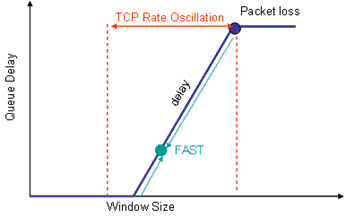
Figure 12 - TCP response function vs FAST
Fast maintains an exponential weighted average RTT measurement and adjusts its window in proportion to the amount by which the current RTT measurement differs from the weighted average RTT measurement. It is harder to provide a graph of a simulation of FAST as compared to the other TCP methods, and the more instructive material has been gather from various experiments using FAST.
XCP - end-to-end and network signalling
It is possible to also call in the assistance of the routers on the path and call on them to mark packets with signalling information relating to current congestion levels. This approach was first explored with the concept of ECN, or Explicit Congestion Notification, and has been generalized into a transport flow control protocol, called “XCP”, where feedback relating to network load is based explicit signals provided by routers relating to their relative sustainable load levels. Interestingly this heads back away from the original design approach of TCP, where the TCP signalling is set up as effectively a heartbeat signal being exchanged by the end systems, and the TCP flow control process is based upon interpretation of the distortions of this heartbeat signal by the network.
XCP appears to be leading into a design approach where the network switching elements play an active role in end-to-end flow control, by effectively signalling to the end systems the current available capacity along the network path. This allows the end systems to respond rapidly to available capacity by increasing the packet rate to the point where the routers along the path signal that no further capacity is available, or to back off the sending rate when the routers along the path signal transient congestion conditions.
Whether such an approach of using explicit router-to-end host signals leads to more efficient very high speed transport protocols remains to be determined, however.
Where next?
The basic question here is whether we’ve reached some form of fundamental limitation of TCP’s window based congestion control protocol, or whether it’s a case that the windows-based control system remains robust at these speeds and distances, but that the manner of control signalling will evolve to adapt to an ever widening range of speed extremes in this environment.
Rate-based pacing, as used in FAST can certainly help with the problem of the problem of guessing what are ‘safe’ window inflation and reduction increments, and it is an open question as to whether its even necessary to use a window inflation and deflation algorithm or whether it would be more effective to head in other directions, such as rate control, RTT stability control or adding additional network-generated information into the high speed control loop. Explicit router-based signalling, such as described in XCP allow for quite precise controls over the TCP session, although what is lost there is the adaptive ability to deploy the control system over any existing IP network.
However, across all these approaches, the basic TCP objectives remain the same: what we want is a transport protocol that can use the available network capacity as efficiently as possible, and as quickly as possible, minimizing the number of retransmissions and maximizing the effective data throughput. What we also want is a protocol that can adapt to other users of the network, and attempt to fairly balance its use with competing claims for network resources.
The various approaches that have been studied to date all represent engineering compromises in one form or another. In attempting to optimise the instantaneous transfer rate the congestion control algorithm may not be responsive to other concurrent transport sessions along the same path. Or in attempting to optimise fairness with other concurrent session the control algorithm may be unresponsive to available network path capacity. The control algorithm may be very unresponsive to dynamic changes in the RTT that may occur during the session due to routing changes in the network path. Which particular metrics of TCP performance are critical in a heterogeneous networking environment is a topic where we have yet to see a clear consensus emerging from the various research efforts.
However, there are a few things we have learned about TCP that form part of this consideration of where to take TCP in this very high speed world:
The first lesson is that TCP has been so effective in terms of overall network efficiency and mutual fairness because everyone uses much the same form of TCP, with very similar response characteristics. If we all elected to use radically different control functions in each of our TCP implementations then it appears likely that we’d have a poorly performing chaotic network subject to extended conditions of complete overload and inefficient network use.
The second lesson is that a transport protocol does not need to solve media level or application issues. The most general form of transport protocol should not rely on characteristics of specific media, but should use specific responses from the lower layers of the protocol stack in order to function correctly as a transport system.
The third lesson from TCP is that a transport protocol can become remarkably persistent and be used in contexts that were simply not considered in the original protocol design, so any design should be careful to allow generous margins of use conditions.
The final lesson is one of fair robustness under competition. Does the protocol negotiate a fair share of the underlying network resource in the face of competing resource claims from concurrent transport flows?
Of all these lessons, the first appears to be the most valuable and probably the hardest to put into practice. The Internet works as well as it does today largely because we all use the much same transport control protocol. If we want to consider some changes to this control protocol to support higher speed flows over extended latency, then it would be perhaps reasonable to see if there is a single control structure and a single protocol that we can all use.
So deciding on a single approach for high speed flows in the high speed internet is perhaps the most critical part of this entire agenda of activity. Its one thing to have a collection of differently controlled packet flows each operating at megabits per second flow rates on a multi-gigabit network, but its quite a frightening prospect to have all kinds of different forms of flows each operating at gigabits per second on the same multi-gigabit network. If we can’t make some progress in reaching a common view of a single high speed TCP control algorithm then it may indeed be the case that none of these approaches will operate efficiently in a highly diverse high speed network environment. So, most importantly, as we do enter into the next generation of very high speed transport protocols it appears that we all need to go together when we go!

![]()
Acknowledgment
I must acknowledge the patient efforts of Larry Dunn in reading through numerous iterations of this article, correcting the text and questioning some of my wilder assertions! Thanks Larry.
However, whatever errors may remain are, undoubtedly, all mine!
![]()
Further Reading
There is a wealth of reading that you can do on this topic, and any decent search engine is your friend here . However if you are interested in this topic then I can recommend the following as a good way to start looking into this topic and gain an overview of the current state of the art in this area:
RFC3649 "HighSpeed TCP for Large Congestion Windows" S. Floyd, December 2003.
-
Sally's treatment of this topic is precise, encompassing
and wonderfully presented. If only all RFC's were of this
quality!
Proceedings of the Workshops on Protocols for Fast Long-Distance Networks
![]()
References
| MulTCP: | “Differentiated end-to-end Internet services using a weighted proportional fair sharing TCP”, J. Crowroft and P. Oechcslin, ACM Computing Communications Review, vol.28, no.3, pp.53–69, July 1998. |
| HighSpeed TCP: | “HighSpeed TCP for Large Congestion Windows”, S. Floyd, RFC 3649, December 2003. |
| Scalable TCP: | “Scalable TCP: Improving Performance in High-Speed Wide Area Networks”, T. Kelly, ACM SIGCOMM Computer Communications Review, Vol. 33, Issue 2, pp 83-91, April 2003. |
| BIC: | “Binary Increase Congestion Control (BIC) for Fast Long-Distance Networks”, L. Xu, K. Harfoush, and I. Rhee, Proceedings of IEEE INFOCOMM 2004, March 2004. |
| CUBIC: | “CUBIC: A New TCP-Friendly High-Speed TCP Variant”, I. Rhee L. Xu, http://www.csc.ncsu.edu/faculty/rhee/export/bitcp/cubic-paper.pdf, February 2005. |
| WESTWOOD: | "TCP Westwood: Congestion Window Control Using Bandwidth Estimation", M. Gerla, M. Y. Sanadidi, R. Wang, A. Zanella, C. Casetti, S. Mascolo, Proceedings of IEEE Globecom 2001, Volume: 3, pp 1698-1702, November 2001. |
| WESTWOOD+: | “Linux 2.4 Implementation of Westwood+ TCP with rate-halving: A Performance Evaluation over the Internet”, A. Dell’Aera, L. A. Greco and S. Mascolo, Tech. Rep. No. 08/03/S, Politecnico di Bari, http://deecal03.poliba.it/mascolo/tcp%20westwood/Tech_Rep_08_03_S.pdf |
| Packet-Pair: | “End-to-end Internet packet dynamics” V. Paxson, Proceedings of ACM SIGCOMM 97, pp 139-152, 1997. |
| H-TCP: | “H-TCP: TCP Congestion Control for High Bandwidth-Delay Product Paths”, D. Leith, R. Shorten, Work in Progress, June 2005 Internet Draft: draft-leith-tcp-htcp-00.txt |
| FAST: | “FAST TCP: Motivation, Architecture, Algorithms, Performance”, C. Jin, X. Wei, and S. H. Low, Proceedings of IEEE INFOCOM 2004, March 2004. |
| XCP: | “Congestion control for high bandwidth-delay product networks”, D. Katabi, M. Handley, and C. Rohrs, ACM Computing Communications Review, vol.32, no.4, pp.89–102, Octpber 2002. |
Geoff Huston
June 2005

Disclaimer
The above views do not necessarily represent the views or positions of the Asia Pacific Network Information Centre, nor those of the Internet Scoiety.
About the Author
GEOFF HUSTON holds a B.Sc. and a M.Sc. from the Australian National University. He has been closely involved with the development of the Internet for the past decade, particularly within Australia, where he was responsible for the initial build of the Internet within the Australian academic and research sector. He is author of a number of Internet-related books. He is the Senior Internet Research Scientist at the Asia Pacific Network Information Centre, the Regional Internet Registry serving the Asia Pacific region.